Propensity score matching for your dissertation: balance, estimands, and APA 7 reporting

of education leadership and policy abstracts name a causal design

7%

in political science

7%

in economics

14%

Many dissertations ask whether a program worked: did mentoring improve first-year persistence, did a professional development model change teaching, did a policy reduce turnover? Most can't randomize who gets the program, and the people who took part usually differ from those who didn't. Propensity score methods address that by comparing participants with nonparticipants who were similar on the characteristics you measured before the program.

Causal designs appear in 7% of method-naming education leadership and policy abstracts, 7% in political science, and 14% in economics in our analysis of recent abstracts. This guide covers what propensity scores can and can't do, the steps from choosing covariates to estimating the effect, example R syntax, how to report the analysis in APA 7, and the questions committees ask.

What a propensity score does

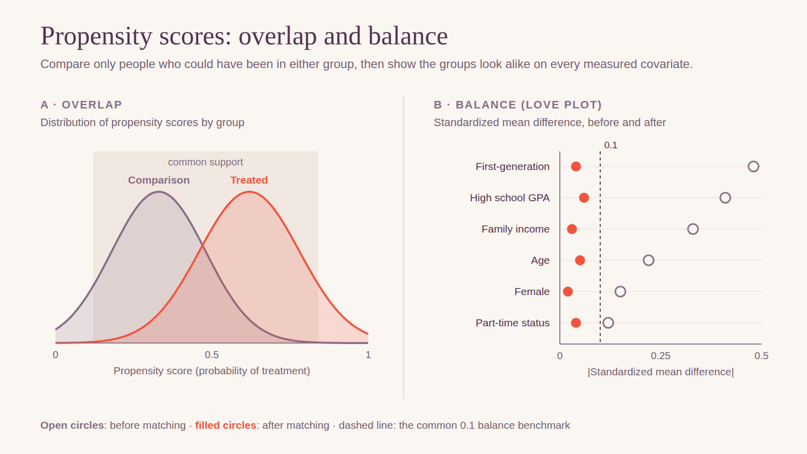
A propensity score is each person's estimated probability of receiving the treatment, given their pre-treatment characteristics (Rosenbaum & Rubin, 1983). People with the same propensity score have, on average, the same distribution of those characteristics whether or not they were treated. Matching or weighting on the score makes the groups comparable on everything that went into it, much as randomization would, but only for the covariates you measured.

That is the central assumption, often called no unmeasured confounding: after accounting for the measured covariates, who received the program is unrelated to how they would have fared. It can't be tested, so the design stands or falls on how well you argue it. Two other conditions matter too: overlap, meaning that treated people have comparable untreated counterparts, and no interference between people, meaning one person's treatment doesn't change another's outcome.

Decide the estimand first

Say which effect you are estimating before you choose a method:

• ATT, the average treatment effect on the treated: how much the program changed outcomes for the people who took it. Matching treated people to similar controls usually targets this.
• ATE, the average treatment effect: how much outcomes would change if everyone in the population received the program versus no one. Inverse probability weighting can target this.

If matching discards treated people who have no good match, the estimate describes only the treated people who were kept. Say so.

Step by step

1. Define the treatment, the outcome, and the timing. Covariates must be measured before treatment.
2. Choose covariates from theory. Include every variable you believe affects both who received the program and the outcome, plus strong predictors of the outcome. Never include variables the program itself could have changed, and avoid variables that predict treatment but not the outcome (Brookhart et al., 2006).
3. Estimate the propensity score, usually with logistic regression. Its coefficients don't matter; its job is to produce balance.
4. Match or weight. Common choices are 1:1 nearest-neighbor matching with a caliper of 0.2 standard deviations of the logit of the propensity score (Austin, 2011), full or optimal matching, and inverse probability weights. Report the ratio, caliper, and whether matching was with replacement.
5. Check overlap and balance. Plot the propensity score distributions and compute standardized mean differences for every covariate before and after. Absolute values below 0.1 are the common benchmark, and variance ratios should be near 1 (roughly 0.5 to 2; Rubin, 2001). Don't use significance tests to judge balance: they depend on sample size, and matching changes it (Imai, King, & Stuart, 2008).
6. Revise until balanced, without looking at the outcome. Add interactions or squared terms to the propensity model, or change the matching method. Keeping this design stage separate from the outcome analysis protects you from choosing the specification that gives the result you hoped for (Rubin, 2001).
7. Estimate the effect in the matched or weighted sample, adjusting for the covariates again for extra protection against leftover imbalance, with standard errors that account for the matching or weighting.
8. Test sensitivity to unmeasured confounding, for example with an E-value (VanderWeele & Ding, 2017): how strong an unmeasured confounder would have to be to explain the effect away.

Running it in R

With MatchIt for matching, cobalt for balance, and marginaleffects for the effect estimate:

library(MatchIt); library(cobalt); library(marginaleffects)

m <- matchit(mentor ~ firstgen + hs_gpa + income + age + female + parttime,
             data = dat, method = "nearest", distance = "glm",
             link = "linear.logit", caliper = 0.2, estimand = "ATT")
summary(m)                                  # balance and sample sizes
love.plot(m, thresholds = c(m = 0.1), abs = TRUE)

md  <- match.data(m)
fit <- glm(persist ~ mentor + firstgen + hs_gpa + income + age + female + parttime,
           data = md, weights = weights, family = quasibinomial)
avg_comparisons(fit, variables = "mentor", vcov = ~subclass,
                newdata = subset(md, mentor == 1), wts = "weights")

The last line gives the ATT as a risk difference, with standard errors clustered on matched pairs. For weighting instead of matching, the WeightIt package works the same way, with cobalt for balance. Stata's teffects psmatch and teffects ipw also estimate these effects, but R's balance diagnostics are the most complete.

Reporting it in APA 7

Report the covariates and why you chose them, the propensity score model, the matching or weighting method with its settings, the estimand, how many people were matched and discarded, a balance table or Love plot with standardized mean differences before and after, the effect with its confidence interval, and the sensitivity analysis. These made-up numbers are internally consistent, so you can use them as a template:

We estimated the effect of peer mentoring on first-year persistence among mentored students (the ATT). Of 1,264 first-year students, 412 were mentored and 852 were not. We estimated propensity scores with logistic regression on six pre-enrollment covariates chosen because prior research links them to both program participation and persistence, and we used 1:1 nearest-neighbor matching without replacement within a caliper of 0.2 standard deviations of the logit of the propensity score (MatchIt; Ho, Imai, King, & Stuart, 2011). Twenty-three mentored students had no match within the caliper and were excluded, leaving 389 matched pairs.

Before matching, absolute standardized mean differences ranged from 0.12 to 0.48; after matching, all were 0.06 or smaller, and variance ratios ranged from 0.91 to 1.08. Among matched students, 84.1% of mentored students persisted, compared with 77.6% of comparison students, a risk difference of 6.5 percentage points, 95% CI [1.2, 11.8], p = .016, with standard errors clustered on matched pairs. An unmeasured confounder would need to be associated with both mentoring and persistence by a risk ratio of 1.39 to explain away this estimate, and by 1.14 to move the confidence interval to include zero (E-values).

Our results chapter guide covers the general APA 7 formatting rules.

Questions committees ask

“Is this as good as a randomized trial?” No. It balances the covariates you measured, and randomization balances everything. Say what you measured, what you couldn't, and what the sensitivity analysis shows about how strong a missing confounder would need to be.

“Why these covariates?” Tie each one to prior research or theory about who selects into the program and what drives the outcome, and confirm that each was measured before treatment.

“Why matching rather than regression adjustment?” Matching or weighting makes the groups comparable in a way you can show, through balance diagnostics, before you look at the outcome, and it makes lack of overlap visible. Regression alone extrapolates across groups that may not overlap.

“You dropped treated people. Who does the result apply to?” To the treated people who had comparable controls. Describe how the excluded people differed.

“Why not use p values to check balance?” Because balance is a property of the sample, not a hypothesis about a population, and p values change with sample size.

“Why propensity score matching at all?” Some methodologists argue that matching on the propensity score alone can increase imbalance when pushed too far (King & Nielsen, 2019). Showing balance directly, and considering full matching or weighting as alternatives, answers this.

Common mistakes

• Claiming causal effects without discussing unmeasured confounding.
• Covariates measured after treatment, or chosen because they are significant predictors of treatment.
• Reporting the propensity model's coefficients instead of balance.
• Judging balance with t tests or p values.
• Trying specifications until the outcome looks good, rather than finishing the design stage first.
• Ignoring the matching when computing standard errors.
• Not naming the estimand, or not saying who was discarded.
• No sensitivity analysis.

Checklist

• Treatment, outcome, timing, and estimand (ATT or ATE) defined
• Covariates justified and all measured before treatment
• Propensity model and matching or weighting method with settings
• Overlap shown, and the number matched and discarded
• Standardized mean differences and variance ratios before and after
• Design finalized before the outcome analysis
• Effect with confidence interval and appropriate standard errors
• Sensitivity analysis for unmeasured confounding
• Causal language matched to the strength of the assumptions

How we did this

The guidance draws on Rosenbaum and Rubin (1983), Biometrika; Rubin (2001), Health Services and Outcomes Research Methodology; Brookhart and colleagues (2006), American Journal of Epidemiology; Imai, King, and Stuart (2008), Journal of the Royal Statistical Society, Series A; Stuart (2010), Statistical Science; Austin (2011), Pharmaceutical Statistics; Ho, Imai, King, and Stuart (2011), Journal of Statistical Software; VanderWeele and Ding (2017), Annals of Internal Medicine; and King and Nielsen (2019), Political Analysis. The shares of abstracts come from our education and social science methods overviews, built from OpenAlex dissertation and thesis abstracts. The analysis code and result tables are on GitHub.

About the author: Dr. Nedim Yel is a statistician with a PhD in measurement, statistics, and methodological studies from Arizona State University. He has led program evaluations for the U.S. Department of Education and nonprofit partners and served on federally funded education research teams.