Exploratory and confirmatory factor analysis for your dissertation: EFA vs. CFA, step by step

of method-naming psychology abstracts describe scale development

6%

in clinical psychology

9%

of teaching and learning abstracts name reliability

25%

Before a committee will trust the relationships in your results chapter, it wants evidence that your scales measure what they claim to. Factor analysis supplies much of that evidence: it shows whether a set of items reflects one construct or several, and which items belong to which. In our analysis of recent abstracts, 6% of method-naming psychology abstracts describe developing a scale, and reliability appears in a quarter of teaching and learning abstracts.

This guide covers the difference between exploratory and confirmatory factor analysis, the decisions in each, example R syntax, how to report both in APA 7, and the questions committees ask most.

EFA or CFA?

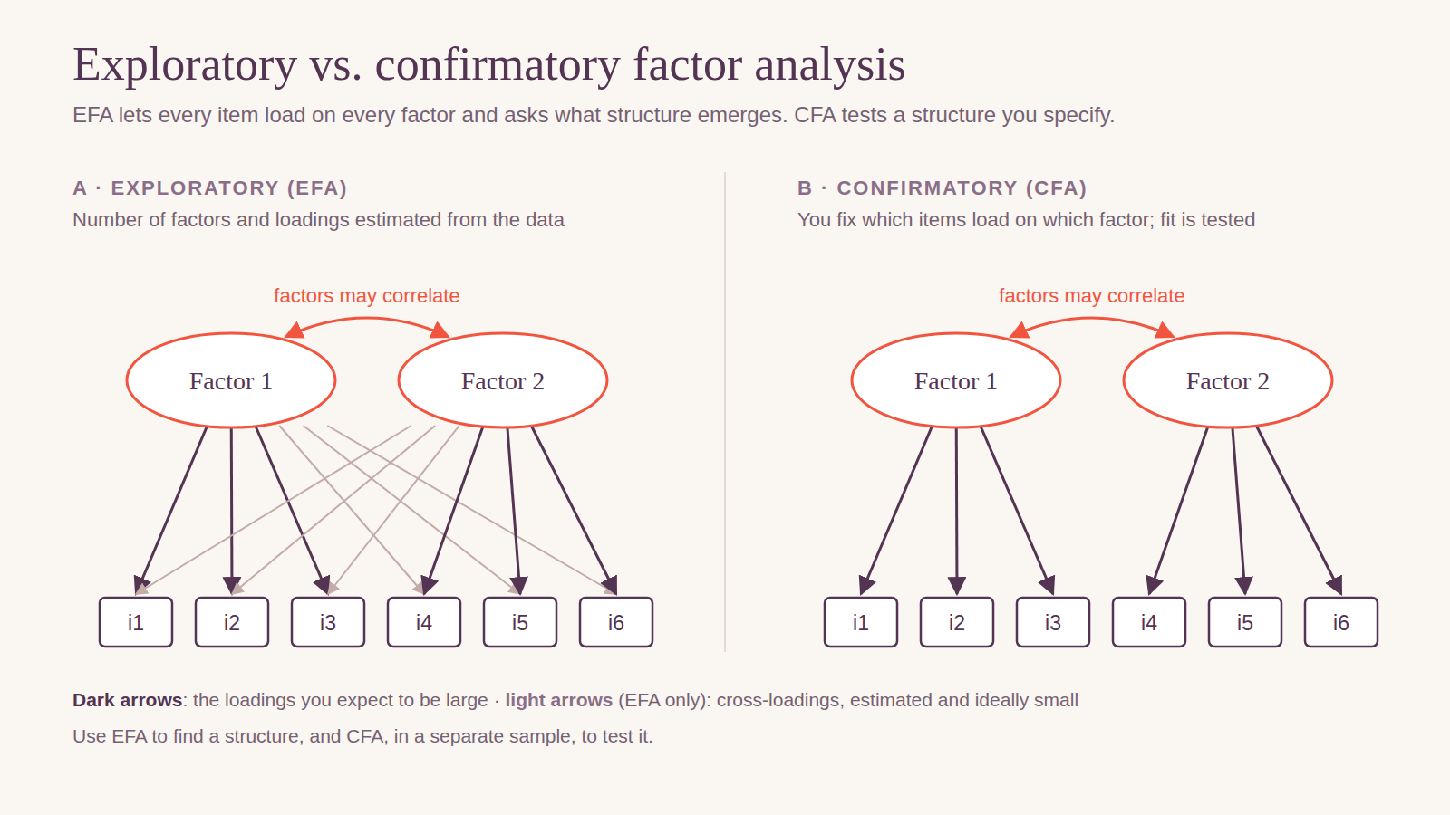
• Exploratory factor analysis (EFA) asks what structure the items have. You don't specify which items belong to which factor. Use it when you are developing a new scale, adapting a scale to a new language or population where its structure is uncertain, or when a published structure has failed to replicate.
• Confirmatory factor analysis (CFA) tests a structure you specify in advance. Use it when you are using an established scale with a known structure, or to test a structure an EFA suggested.

Don't run EFA and CFA on the same data and call the CFA a confirmation: the CFA will fit the structure the EFA found in that same sample. If you need both, split the sample randomly, or collect a second sample.

EFA, step by step

1. Check that the data can be factored. Report the Kaiser–Meyer–Olkin measure (values of about .60 or higher are usually acceptable, and .80 or higher is good) and Bartlett's test of sphericity, which should be significant. Look for items that correlate weakly with all the others.
2. Choose the correlations. For Likert items with few response categories, polychoric correlations describe the items better than Pearson correlations.
3. Choose an extraction method. Principal axis factoring, minimum residuals, or maximum likelihood. Principal components analysis is not factor analysis: it summarizes total variance rather than modeling the shared variance a latent construct explains (Fabrigar, Wegener, MacCallum, & Strahan, 1999).
4. Decide how many factors to keep. Parallel analysis (Horn, 1965), which compares your eigenvalues with those from random data, is the best-supported criterion. The “eigenvalue greater than 1” rule tends to keep too many factors, so don't use it alone. Check that the solution you pick makes theoretical sense, and compare it with one more and one fewer factor.
5. Rotate obliquely. Constructs in the social sciences usually correlate, so use an oblique rotation such as oblimin or promax. Varimax forces the factors to be uncorrelated. If the factors really are unrelated, an oblique rotation will show that.
6. Interpret the pattern matrix. With an oblique rotation, interpret the pattern coefficients. Loadings of about .40 or higher are a common benchmark, items loading above about .30 on two factors are flagged as cross-loading, and each factor should have at least three items.
7. Remove items one at a time, with reasons. Drop a weak or cross-loading item only after checking its content, rerun the EFA after each removal, and report every item you removed and why.

Sample size. Rules such as ten cases per item are unreliable. MacCallum, Widaman, Zhang, and Hong (1999) showed that the sample needed depends mostly on communalities and on how many items each factor has: with high communalities and several items per factor, samples near 100 can work, while low communalities call for several hundred.

CFA, step by step

1. Specify the model from theory or from an earlier EFA: which items load on which factor, and whether the factors correlate.
2. Choose the estimator. With five or more response categories and roughly symmetric items, robust maximum likelihood (MLR) works well. With fewer categories or strongly skewed items, treat items as ordinal and use WLSMV (Rhemtulla, Brosseau-Liard, & Savalei, 2012).
3. Judge fit with χ², CFI, TLI, RMSEA with its 90% confidence interval, and SRMR, and check local fit through residual correlations. Our SEM guide explains each index and why cutoffs are guidelines rather than rules.
4. Change the model only for substantive reasons, such as two items with nearly identical wording, and report every change.
5. Report reliability and validity evidence: standardized loadings, omega for each factor, and evidence that the factors are distinct, such as average variance extracted or heterotrait–monotrait ratios.
6. Test measurement invariance if you will compare groups. Configural, metric, and scalar invariance show that the scale means the same thing across groups before you compare their scores.

Running it in R

EFA with the psych package, on polychoric correlations:

library(psych)
KMO(items)
cortest.bartlett(cor(items), n = nrow(items))
fa.parallel(items, fm = "pa", fa = "fa", cor = "poly")
efa <- fa(items, nfactors = 3, fm = "pa", rotate = "oblimin", cor = "poly")
print(efa, cut = .30, sort = TRUE)

CFA with lavaan, treating the items as ordinal (WLSMV is lavaan's default for ordered items):

library(lavaan)
model <- '
  support  =~ i1 + i2 + i3 + i4 + i5 + i6
  autonomy =~ i7 + i8 + i9 + i10 + i11
  workload =~ i12 + i13 + i14 + i15 + i16
'
fit <- cfa(model, data = cfa_half, ordered = paste0("i", 1:16))
summary(fit, fit.measures = TRUE, standardized = TRUE)
semTools::compRelSEM(fit)   # omega for each factor

In SPSS, EFA is under Analyze > Dimension Reduction > Factor. Change the extraction method from the default, principal components, to principal axis factoring, and the rotation to direct oblimin or promax. SPSS has no built-in parallel analysis; O'Connor's (2000) syntax or R can run it.

Reporting it in APA 7

For an EFA, report the sample, the KMO and Bartlett's test, the correlations, extraction method, and rotation, how you decided the number of factors, the variance explained, a table of pattern coefficients and communalities, the factor correlations, and every item you removed and why. For a CFA, report the model, software, estimator, missing-data handling, fit indices, standardized loadings, reliability, and any modifications. These made-up numbers are internally consistent, so you can use them as a template:

We randomly split the sample into an exploratory half (n = 320) and a confirmatory half (n = 318). In the exploratory half, the 18 items were suitable for factor analysis, KMO = .89, Bartlett's χ²(153) = 3,412.6, p < .001. Parallel analysis on polychoric correlations suggested three factors. We extracted three factors with principal axis factoring and oblimin rotation. Two items loaded above .30 on two factors and were removed, one at a time. In the final 16-item solution, pattern coefficients on the primary factors ranged from .48 to .86, no cross-loading exceeded .25, the three factors explained 52% of the variance in the items, and factor correlations ranged from .31 to .52.

In the confirmatory half, we tested the three-factor structure with WLSMV estimation in lavaan (Rosseel, 2012). The model fit well, χ²(101) = 212.4, p < .001, CFI = .98, TLI = .98, RMSEA = .059, 90% CI [.048, .070], SRMR = .051. Standardized loadings ranged from .62 to .91, all p < .001, and omega reliability was .84, .87, and .90 for the three factors.

Put the pattern coefficients and the CFA loadings in tables rather than the text. Our results chapter guide covers the general APA 7 formatting rules.

Questions committees ask

“Why not principal components analysis?” PCA summarizes all the variance in the items, including error, into components. Factor analysis models the shared variance that a construct explains, which is the question when you are validating a scale.

“How did you decide on the number of factors?” Name the criteria, led by parallel analysis, and show that the chosen solution is interpretable and better than the solutions with one more or one fewer factor.

“Why oblique rotation?” Because the constructs are expected to correlate, and an oblique rotation lets them. Report the factor correlations.

“This is an established scale. Why did you run an EFA?” Usually you shouldn't: test the published structure with a CFA. An EFA is justified when the scale is new to your population or language, or when the CFA fits poorly and you need to see why.

“You dropped items. Does the scale still measure the whole construct?” Show what each removed item asked and check that the remaining items still cover the construct's definition. Say whether scores were computed with the original or reduced item set.

“Why omega rather than Cronbach's alpha?” Alpha assumes every item is equally related to the construct, which CFA loadings rarely show. Omega uses the actual loadings (McNeish, 2018). Many committees still expect alpha too, so report both.

Common mistakes

• Running PCA with the eigenvalue-greater-than-1 rule and varimax, the SPSS defaults, and calling it factor analysis.
• EFA and CFA on the same sample, reported as confirmation.
• An EFA on an established scale where a CFA was the right test.
• Pearson correlations and maximum likelihood on three- or four-category items without considering an ordinal approach.
• Interpreting the structure matrix after an oblique rotation instead of the pattern matrix.
• Dropping many items at once, or without reporting which and why.
• Reporting only fit, or only alpha, without loadings.
• Comparing group means without testing measurement invariance.

Checklist

• Choice of EFA, CFA, or both justified, with separate samples for each
• Sample size discussed in terms of communalities and items per factor
• EFA: KMO, Bartlett's test, correlation type, extraction, and rotation reported
• Number of factors chosen with parallel analysis and interpretability
• Pattern coefficient table with communalities and factor correlations
• Every removed item listed with its reason
• CFA: estimator, fit indices, standardized loadings, and modifications
• Omega (and alpha, if expected) for each factor
• Measurement invariance tested before comparing groups

How we did this

The guidance draws on Fabrigar, Wegener, MacCallum, and Strahan (1999), Psychological Methods; Horn (1965), Psychometrika; MacCallum, Widaman, Zhang, and Hong (1999), Psychological Methods; Rhemtulla, Brosseau-Liard, and Savalei (2012), Psychological Methods; O'Connor (2000), Behavior Research Methods, Instruments, & Computers; and McNeish (2018), Psychological Methods. The shares of abstracts come from our psychology and education methods overviews, built from OpenAlex dissertation and thesis abstracts. The analysis code and result tables are on GitHub.

About the author: Dr. Nedim Yel is a statistician with a PhD in measurement, statistics, and methodological studies from Arizona State University. He has published factor-analytic and measurement research, including in School Psychology and the Journal of Educational Measurement.