
- of method-naming marketing abstracts name SEM
- 24%
- across business dissertations
- 12%
- of SEM abstracts report a confidence interval
- 1%
Structural equation modeling (SEM) tests a set of relationships among constructs, such as leadership, psychological safety, and engagement, while modeling how each construct was measured. It is a mainstay of business, psychology, and education dissertations. In our analysis of recent abstracts, SEM appears in 24% of method-naming marketing abstracts and 12% across business.
SEM rewards careful planning and punishes shortcuts: the sample size, the item scales, the estimator, and every change to the model all end up in front of your committee. This guide covers the two parts of a model, the decisions to make before you run it, example syntax, how to judge fit, how to report results in APA 7, and the questions committees ask.
Two models in one
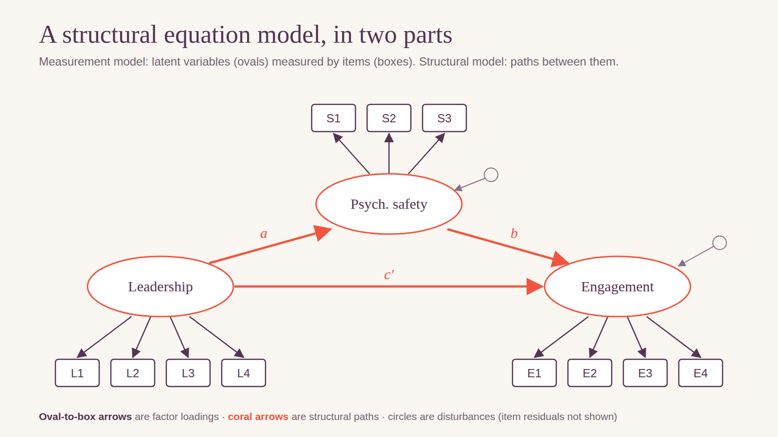
Every SEM has a measurement model, which says which items measure which latent variable (a confirmatory factor analysis, or CFA), and a structural model, which says how the latent variables relate. Because each construct is estimated from several items, the structural paths are corrected for measurement error, which regression on scale averages can't do. A model with only observed variables and no measurement part is a path analysis.
Most dissertations follow Anderson and Gerbing's (1988) two-step approach: first fit the measurement model alone and make sure it holds, then add the structural paths. If the measurement model fits poorly, the structural results can't be trusted, and problems are much easier to find before the structural paths are added.
Decisions to make before you run it
- Sample size. Rules of thumb such as “200 cases” or “10 cases per parameter” are unreliable. Wolf and colleagues (2013) found that the sample needed ranged from about 30 to 460 depending on the number of factors, indicators, loadings, and missing data. The defensible approach is a Monte Carlo power analysis for your model; our power analysis guide covers how to plan and justify it.
- Indicators. Aim for at least three items per latent variable. Two-item factors often cause estimation problems.
- Item scales and estimator. With five or more response categories and roughly symmetric items, robust maximum likelihood (MLR) works well (Rhemtulla, Brosseau-Liard, & Savalei, 2012). With fewer categories or strongly skewed items, treat items as ordinal and use WLSMV.
- Missing data. Full-information maximum likelihood (FIML) uses every case's available data. Report how much was missing and why you think it's missing at random.
- Identification. Each latent variable needs a scale: fix one loading to 1 (the default in most software) or fix the factor's variance to 1.
- Theory first. Write down every path and its rationale before you see the data. Committees distinguish sharply between hypothesized paths and ones added later.
Running it
SEM runs in R (lavaan), Mplus, AMOS, and Stata. Here is the model in the figure in lavaan, with MLR and FIML:
library(lavaan)
model <- '
  # measurement model
  lead   =~ l1 + l2 + l3 + l4
  safety =~ s1 + s2 + s3
  engage =~ e1 + e2 + e3 + e4
  # structural model
  safety ~ a*lead
  engage ~ b*safety + cp*lead
  indirect := a*b
  total    := cp + a*b
'
fit <- sem(model, data = survey, estimator = "MLR", missing = "fiml")
summary(fit, fit.measures = TRUE, standardized = TRUE, rsquare = TRUE)
For the indirect effect, refit with maximum likelihood and bootstrap standard errors, and report percentile bootstrap intervals:
set.seed(31216)
fit_boot <- sem(model, data = survey, missing = "fiml",
                se = "bootstrap", bootstrap = 5000)
parameterEstimates(fit_boot, boot.ci.type = "perc", standardized = TRUE)
The same model in Mplus:
MODEL:    lead BY l1-l4;
          safety BY s1-s3;
          engage BY e1-e4;
          safety ON lead;
          engage ON safety lead;
MODEL INDIRECT:
          engage IND lead;
OUTPUT:   STANDARDIZED;
To fit step one, the measurement model alone, replace the structural lines with correlations among the factors (lavaan does this by default when you leave them out; Mplus does too).
Judging fit
SEM asks whether the model reproduces the relationships among your items. Report several indices, because each captures something different:
- Chi-square (χ²) with its degrees of freedom and p value. It tests exact fit and becomes significant for trivial misfit in large samples, so it is reported but rarely decisive. With MLR, report the scaled chi-square.
- CFI and TLI, comparing your model with a model of no relationships. Values of about .95 or higher are commonly read as good fit.
- RMSEA with its 90% confidence interval, the misfit per degree of freedom. About .06 or lower is commonly read as good.
- SRMR, the average residual correlation. About .08 or lower is commonly read as good.
These benchmarks come from Hu and Bentler (1999), whose own simulations covered a limited set of models. Marsh, Hau, and Wen (2004) warn against treating them as pass-or-fail rules, and they are more lenient or strict depending on the model. Treat them as guidelines, and also check local fit: large residual correlations between specific items tell you where the model misses, even when the overall indices look fine.
When fit is poor: changing the model
Modification indices estimate how much chi-square would drop if you freed a parameter, most often a correlation between two items' residuals or a cross-loading. Used freely, they fit the model to your sample's quirks. Change the model only when the change has a substantive reason (for example, two items share wording or a method), make one change at a time, and report every change with its rationale. Say clearly that modified models are exploratory, and, if your sample is large enough, confirm them in a holdout half.
Reporting the measurement model
For each latent variable, report the standardized loadings (usually in a table), reliability (omega or composite reliability), and evidence that the constructs are distinct. Common evidence of distinctness is average variance extracted (AVE) of at least .50 with each factor's AVE exceeding its squared correlations with the other factors (Fornell & Larcker, 1981), or heterotrait–monotrait ratios (HTMT) below .85 or .90 (Henseler, Ringle, & Sarstedt, 2015). If you compare groups, test measurement invariance (configural, metric, then scalar) before comparing their paths or means.
Reporting it in APA 7
APA's reporting standards (JARS–Quant) include a module for SEM. Report the model specification with a diagram, the software and estimator, missing-data handling, sample size, fit indices for each model you fit, the loadings, the structural paths with standard errors or confidence intervals, R² for each outcome, indirect effects with bootstrap intervals, every modification, and the correlation or covariance matrix (usually in an appendix). These made-up numbers are internally consistent, so you can use them as a template:
We tested the hypothesized model in two steps (Anderson & Gerbing, 1988) in lavaan 0.6 (Rosseel, 2012), using robust maximum likelihood with full-information handling of missing data (N = 412). The three-factor measurement model fit the data well, χ²(41) = 98.6, p < .001, CFI = .96, TLI = .95, RMSEA = .058, 90% CI [.043, .073], SRMR = .045. Standardized loadings ranged from .68 to .87 (all p < .001), omega reliability from .82 to .89, and AVE from .52 to .64, and all HTMT ratios were below .61.
Because the structural model estimated all three paths among the factors, its fit was identical to that of the measurement model. Transformational leadership was positively associated with psychological safety, β = .48, 95% CI [.39, .57], and psychological safety with engagement, β = .36, 95% CI [.25, .47]. Leadership was also directly associated with engagement, β = .21, 95% CI [.09, .33]. The standardized indirect effect of leadership on engagement through psychological safety was .17, 95% percentile bootstrap CI [.11, .24], based on 5,000 resamples. The model explained 23% of the variance in psychological safety and 25% in engagement.
A table of standardized loadings and a path diagram with the standardized coefficients let readers check the text. Our results chapter guide covers the general APA 7 formatting rules, and the PROCESS mediation guide explains indirect effects in more detail.
Questions committees ask
“Why SEM instead of regression on scale scores?” SEM models measurement error, so the relationships among constructs are not weakened by unreliable items, and it tests the whole model at once, with fit indices that tell you whether it is consistent with the data.
“Is your sample large enough?” Answer with a Monte Carlo power analysis or a sensitivity analysis for your model, not a rule of thumb.
“Your fit is borderline. What does that mean?” Report all the indices, show where the model misfits locally, and explain what that implies for the paths you interpret. Don't claim good fit from the one index that passes.
“Didn't you just modify the model until it fit?” Show that each change had a substantive reason, report the original and final models, and label the final model as partly exploratory.
“Couldn't a different model fit just as well?” Often yes. Equivalent models, such as reversing a path, can fit exactly as well (MacCallum, Wegener, Uchino, & Fabrigar, 1993). Name the plausible alternatives and argue for yours from theory and design, not from fit.
“Does SEM show causation?” No more than regression does. Arrows state your causal hypothesis; the data can be consistent with it, but the design determines what you can conclude.
“Why covariance-based SEM rather than PLS-SEM, or the reverse?” PLS-SEM, common in marketing and information systems, builds constructs as weighted composites and aims at prediction. Covariance-based SEM treats constructs as common factors and tests model fit. Choose the one that matches how you think your constructs relate to their items, and expect committees and reviewers in some fields to question PLS used mainly because the sample is small.
Common mistakes
- Skipping the measurement model and interpreting structural paths from a poorly fitting model.
- Reporting one fit index, or only the ones that look good.
- Chasing modification indices without a substantive reason, or making changes without reporting them.
- Using maximum likelihood on three- or four-category items without considering an ordinal estimator.
- Listwise deletion when FIML is available.
- Standardized paths without uncertainty. Report standard errors or confidence intervals, and bootstrap intervals for indirect effects.
- No diagram and no correlation matrix, so readers can't check or reproduce the model.
- Causal language the design can't support.
Checklist
- Model and every path specified with a theoretical rationale before analysis
- Sample-size justification for the model
- Software, version, and estimator named, with the reason for the estimator
- Missing-data amount and handling reported
- Measurement model fit, loadings, reliability, and construct distinctness
- Structural model fit: χ² with df, CFI, TLI, RMSEA with 90% CI, and SRMR
- Structural paths with SEs or CIs, and R² for each outcome
- Indirect effects with bootstrap CIs, number of resamples, and seed
- Every model modification and its rationale
- Path diagram, loadings table, and correlation matrix
How we did this
The guidance draws on Kline's Principles and Practice of Structural Equation Modeling (5th ed., Guilford Press, 2023), APA's JARS–Quant standards, and the studies cited above: Anderson and Gerbing (1988), Psychological Bulletin; Hu and Bentler (1999), Structural Equation Modeling; Marsh, Hau, and Wen (2004), Structural Equation Modeling; Wolf, Harrington, Clark, and Miller (2013), Educational and Psychological Measurement; Rhemtulla, Brosseau-Liard, and Savalei (2012), Psychological Methods; Fornell and Larcker (1981), Journal of Marketing Research; Henseler, Ringle, and Sarstedt (2015), Journal of the Academy of Marketing Science; and MacCallum and colleagues (1993), Psychological Bulletin. The shares of abstracts naming SEM come from our business methods overview, and the reporting rate from the same 112,903 OpenAlex dissertation and thesis abstracts as our results chapter guide. The analysis code and result tables are on GitHub.